Decoding Algorithm Efficiency: A Guide to Big O Notation

Introduction

Big O notation helps evaluate algorithm efficiency independent of hardware or software. Because real-world runtime comparisons (in seconds or minutes) are unreliable due to variations in hardware and software, asymptotic complexity analyzes how an algorithm’s runtime scales with increasing input size (n). Big-O notation provides an upper bound on the growth rate of an algorithm’s resource usage (time or space).

Key Concepts:

• Input Size (n): The primary factor influencing an algorithm’s performance. This could be the number of elements in an array, the number of nodes in a graph, etc.
• Runtime: The time taken for an algorithm to complete its execution.
• Space Complexity: The amount of memory an algorithm uses.
• Asymptotic Analysis: Analyzing algorithm performance as the input size grows towards infinity, focusing on the dominant factors and ignoring constant factors and lower-order terms.

Visualizing Growth Rates

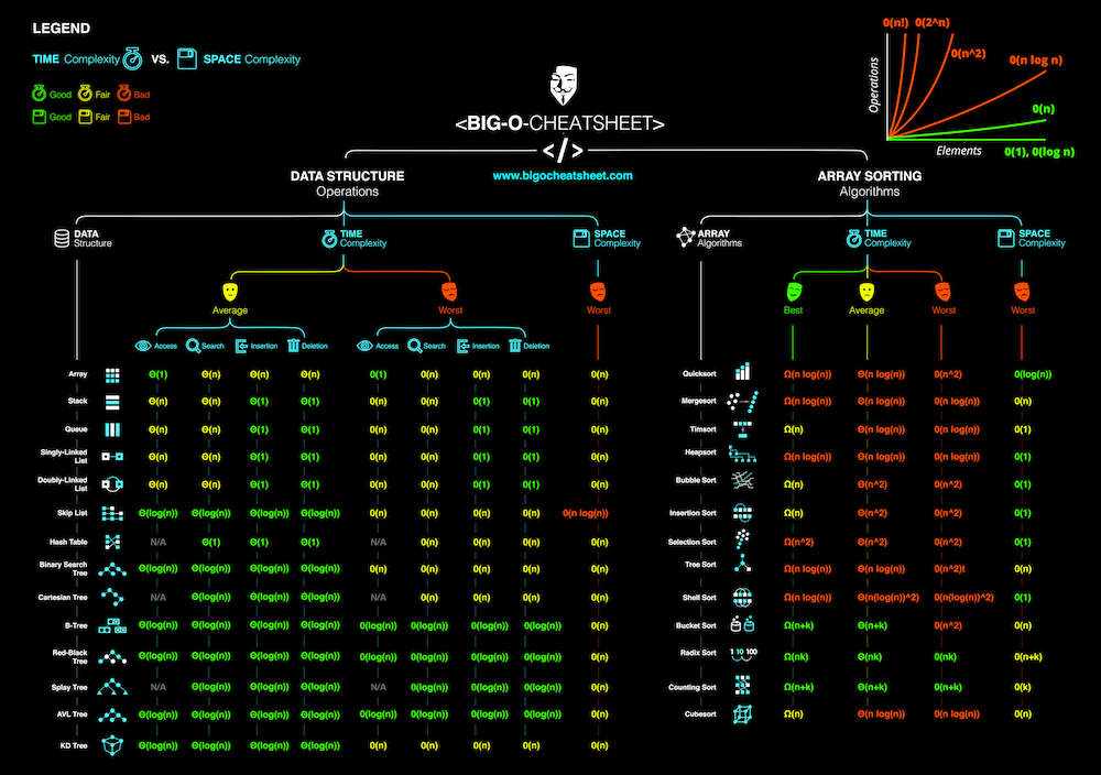(showing the growth rates of common Big O complexities: O(1), O(log n), O(n), O(n log n), O(n^2), O(2^n), O(n!))

Common Big O Complexities with Code Examples

Here are some common Big O complexities with illustrative code examples:

• O(1) - Constant Time: The algorithm’s runtime doesn’t change as the input size grows.

    // Example: Accessing an element in an array by its index.
    int getElementAtIndex(int[] arr, int index) {
        return arr[index];
    }
  

• O(log n) - Logarithmic Time: The runtime increases logarithmically with the input size.

    // Example: Binary search in a sorted array.
    int binarySearch(int[] arr, int target) {
        int low = 0, high = arr.length - 1;
        while (low <= high) {
            int mid = low + (high - low) / 2;
            if (arr[mid] == target) return mid;
            if (arr[mid] < target) low = mid + 1;
            else high = mid - 1;
        }
        return -1; // Not found
    }
  

• O(n) - Linear Time: The runtime increases linearly with the input size.

    // Example: Iterating through an array to find an element.
    int linearSearch(int[] arr, int target) {
        for (int i = 0; i < arr.length; i++) {
            if (arr[i] == target) return i;
        }
        return -1; // Not found
    }
  

• O(n log n) - Linearithmic Time: The runtime increases proportionally to n multiplied by the logarithm of n.

    // Example: Merge sort (a common sorting algorithm).
    // (Merge sort is a bit more complex to show concisely,
    //  but you can find many implementations online)
    void mergeSort(int[] arr, int l, int r) {
        if (l < r) {
            int m = l + (r - l) / 2;
            mergeSort(arr, l, m);
            mergeSort(arr, m + 1, r);
            // Merge the sorted subarrays (implementation omitted for brevity)
        }
    }
  

• O(n^2) - Quadratic Time: The runtime increases proportionally to the square of the input size.

    // Example: Nested loops iterating over an array (e.g., bubble sort).
    void bubbleSort(int[] arr) {
        for (int i = 0; i < arr.length; i++) {
            for (int j = 0; j < arr.length - i - 1; j++) {
                if (arr[j] > arr[j + 1]) {
                    // Swap arr[j] and arr[j+1]
                    int temp = arr[j];
                    arr[j] = arr[j + 1];
                    arr[j + 1] = temp;
                }
            }
        }
    }
  

• O(2^n) - Exponential Time: The runtime doubles with each addition to the input size.

    // Example: Recursive Fibonacci calculation (naive implementation).
    int fibonacci(int n) {
        if (n <= 1) return n;
        return fibonacci(n - 1) + fibonacci(n - 2);
    }
  

• O(n!) - Factorial Time: The runtime grows factorially with the input size.

    // Example: Traveling Salesperson Problem (brute-force approach, very inefficient).
    // (A full implementation is quite complex, so this is just a conceptual illustration)
    void travelingSalesperson(City[] cities, Route currentRoute) {
        if (all cities visited) {
            evaluateRoute(currentRoute);
        } else {
            for each unvisited city {
                travelingSalesperson(cities, currentRoute + city);
            }
        }
    }
  

How to Determine Big O: A Step-by-Step Guide

1. Identify the dominant operations: Focus on the operations that contribute most significantly to the runtime as n grows. These are often found within loops or recursive calls.
2. Express the number of operations in terms of n:
   • Loops:
     • A single loop that iterates n times is typically O(n).
     • Nested loops, where each loop iterates n times, are typically O(n^2), O(n^3), etc., depending on the nesting depth.
     • Loops where the counter is multiplied or divided by a constant in each iteration are often O(log n) (like in binary search).
   • Recursive Functions: Analyze the number of recursive calls and the work done in each call. Techniques like drawing a recursion tree or using the Master Theorem (for simple cases) can help.
3. Use Big-O notation to represent the growth rate:
   • Dominant Term: Keep only the term with the highest growth rate. For example, if you have n^2 + n, the dominant term is n^2, so the Big O is O(n^2).
   • Ignore Constant Factors: Drop constant multipliers. O(2n) simplifies to O(n). As the input size becomes very large, the constant factor becomes less significant compared to the growth rate of n.

Best, Average, and Worst-Case Analysis

An algorithm’s performance can vary depending on the specific input. Therefore, we often consider:

• Best-Case: The scenario where the algorithm performs most efficiently. Often less informative because it might not represent typical usage.
• Average-Case: The expected performance for typical input. Can be challenging to calculate accurately.
• Worst-Case: The scenario where the algorithm performs least efficiently. Provides an upper bound on the runtime and is often the most important for practical purposes because it guarantees the algorithm won’t perform worse than this.

Why Big O Matters

• Algorithm Selection: Choosing the most efficient algorithm for a given task can significantly impact performance, especially for large datasets.
• Performance Prediction: Estimating how an algorithm will perform with larger datasets allows for better planning and resource allocation.
• Code Optimization: Identifying performance bottlenecks and improving code efficiency by focusing on parts of the code with high time complexity.

Beyond Big O: A More Complete Picture

While Big O provides an upper bound, a more comprehensive analysis might involve:

• Big Omega (Ω): Represents the lower bound on the growth rate of an algorithm. It describes the best-case scenario or the minimum amount of resources (time or space) the algorithm will require.
• Big Theta (Θ): Represents a tight bound on the growth rate. It means that the algorithm’s runtime grows at the same rate as the function within the Θ notation. We can use Big Theta when the upper and lower bounds are the same.

Example:

Consider an algorithm that always takes exactly 3n + 5 steps, regardless of the input.

• Big O: We can say it’s O(n) because 3n + 5 is less than or equal to 4n for sufficiently large n.
• Big Omega: We can also say it’s Ω(n) because 3n + 5 is greater than or equal to 3n for all n.
• Big Theta: Since the upper and lower bounds are both n, we can say the algorithm’s complexity is Θ(n). This indicates that the algorithm’s runtime grows linearly with the input size, precisely.

Amortized Analysis: Understanding Average Performance

Amortized analysis is a technique used to analyze algorithms that have occasional expensive operations, but where the average cost of operations over time is lower. A classic example is the dynamic array.

• Dynamic Arrays: These are arrays that automatically resize themselves when they become full. Resizing typically involves allocating a new, larger array and copying the elements from the old array to the new one. This copying operation takes O(n) time.
• Amortized O(1) Insertion: However, resizing doesn’t happen on every insertion. Most insertions into a dynamic array are very fast (O(1) because they just involve adding an element to the end). When we consider the average cost of insertions over a long sequence of operations, including the occasional expensive resizing operations, the amortized cost per insertion is still O(1).

Algorithm Comparison: When Big O Isn’t Everything

While Big O notation is a powerful tool, it’s essential to remember that it’s not the only factor to consider when comparing algorithms:

• Constant Factors: For smaller input sizes, constant factors that are ignored in Big O notation can play a significant role. An algorithm with a worse Big O complexity might outperform another algorithm with a better Big O complexity if its constant factors are much smaller.
• Example:
  • Algorithm A has a runtime of 1000n.
  • Algorithm B has a runtime of 10n^2. Big O would suggest that Algorithm A (O(n)) is better than Algorithm B (O(n^2)). However, if n is less than 100, Algorithm B will be faster.
• Practical Considerations:
  • Code Readability and Maintainability: Sometimes, a slightly less efficient algorithm might be preferred if it’s significantly simpler to understand, implement, and maintain.
  • Specific Input Characteristics: If you have knowledge about the specific characteristics of your input data, you might be able to choose an algorithm that is optimized for those characteristics, even if its general Big O complexity is not the best.

Conclusion

By understanding algorithmic complexity and Big-O notation, you can make informed decisions about algorithm selection and optimize your code for better performance. Remember to consider not just the Big O complexity but also constant factors, code readability, and the specific characteristics of your data when making choices about algorithms.

Practice Makes Perfect

The best way to solidify your understanding of Big O notation is to practice! Try determining the Big O complexity of different code snippets or algorithms. Websites like LeetCode, HackerRank, and similar platforms offer a wealth of algorithmic problems where you can apply your knowledge. You can also experiment with different algorithms and input sizes to see how their performance changes in practice.